Toggle navigation

.rst .pdf

Contents

Hyper Parameter Search

Tools to perform hyperparameter optimization of Scikit-Learn API-compatible models using Dask, and to scale hyperparameter optimization to larger data and/or larger searches.

Hyperparameter searches are a required process in machine learning. Briefly, machine learning models require certain “hyperparameters”, model parameters that can be learned from the data. Finding these good values for these parameters is a “hyperparameter search” or an “hyperparameter optimization.” For more detail, see “Tuning the hyper-parameters of an estimator.”

These searches can take an ample time (days or weeks), especially when good performance is desired and/or with massive datasets, which is common when preparing for production or a paper publication. The following section clarifies the issues that can occur:

• “Scaling hyperparameter searches” mentions problems that often occur in hyperparameter optimization searches.

Tools that address these problems are expanded upon in these sections:

1. “Drop-In Replacements for Scikit-Learn” details classes that mirror the Scikit-learn estimators but work nicely with Dask objects and can offer better performance.

2. “Incremental Hyperparameter Optimization” details classes that work well with large datasets.

3. “Adaptive Hyperparameter Optimization” details classes that avoid extra computation and find high-performing hyperparameters more quickly.

Scaling hyperparameter searches

Dask-ML provides classes to avoid the two most common issues in hyperparameter optimization, when the hyperparameter search is…

1. “memory constrained”. This happens when the dataset size is too large to fit in memory. This typically happens when a model needs to be tuned for a larger-than-memory dataset after local development.

2. “compute constrained”. This happen when the computation takes too long even with data that can fit in memory. This typically happens when many hyperparameters need to be tuned or the model requires a specialized hardware (e.g., GPUs).

“Memory constrained” searches happen when the data doesn’t fit in the memory of a single machine:

>>> import pandas as pd
>>> import dask.dataframe as dd
>>>
>>> ## not memory constrained
>>> df = pd.read_csv("data/0.parquet")
>>> df.shape
(30000, 200)  # => 23MB
>>>
>>> ## memory constrained
>>> # Read 1000 of the above dataframes (=> 22GB of data)
>>> ddf = dd.read_parquet("data/*.parquet")

“Compute constrained” is when the hyperparameter search takes too long even if the data fits in memory. There might a lot of hyperparameters to search, or the model may require specialized hardware like GPUs:

>>> import pandas as pd
>>> from scipy.stats import uniform, loguniform
>>> from sklearn.linear_model import SGDClasifier
>>>
>>> df = pd.read_parquet("data/0.parquet")  # data to train on; 23MB as above
>>>
>>> model = SGDClasifier()
>>>
>>> # not compute constrained
>>> params = {"l1_ratio": uniform(0, 1)}
>>>
>>> # compute constrained
>>> params = {
...     "l1_ratio": uniform(0, 1),
...     "alpha": loguniform(1e-5, 1e-1),
...     "penalty": ["l2", "l1", "elasticnet"],
...     "learning_rate": ["invscaling", "adaptive"],
...     "power_t": uniform(0, 1),
...     "average": [True, False],
... }
>>>

These issues are independent and both can happen the same time. Dask-ML has tools to address all 4 combinations. Let’s look at each case.

Neither compute nor memory constrained

This case happens when there aren’t many hyperparameters to tune and the data fits in memory. This is common when the search doesn’t take too long to run.

Scikit-learn can handle this case:

sklearn.model_selection.GridSearchCV(...[, ...])	Exhaustive search over specified parameter values for an estimator.
sklearn.model_selection.RandomizedSearchCV(...)	Randomized search on hyper parameters.

Dask-ML also has some drop in replacements for the Scikit-learn versions that works well with Dask collections (like Dask Arrays and Dask DataFrames):

dask_ml.model_selection.GridSearchCV(...[, ...])	Exhaustive search over specified parameter values for an estimator.
dask_ml.model_selection.RandomizedSearchCV(...)	Randomized search on hyper parameters.

By default, these estimators will efficiently pass the entire dataset to fit if a Dask Array/DataFrame is passed. More detail is in “Works Well With Dask Collections”.

These estimators above work especially well with models that have expensive preprocessing, which is common in natural language processing (NLP). More detail is in “Compute constrained, but not memory constrained” and “Avoid Repeated Work”.

Memory constrained, but not compute constrained

This case happens when the data doesn’t fit in memory but there aren’t many hyperparameters to search over. The data doesn’t fit in memory, so it makes sense to call partial_fit on each chunk of a Dask Array/Dataframe. This estimator does that:

dask_ml.model_selection.IncrementalSearchCV(...)

Incrementally search for hyper-parameters on models that support partial_fit

More detail on IncrementalSearchCV is in “Incremental Hyperparameter Optimization”.

Dask’s implementation of GridSearchCV and RandomizedSearchCV can to also call partial_fit on each chunk of a Dask array, as long as the model passed is wrapped with Incremental.

Compute constrained, but not memory constrained

This case happens when the data fits in the memory of one machine but when there are a lot of hyperparameters to search, or the models require specialized hardware like GPUs. The best class for this case is HyperbandSearchCV:

dask_ml.model_selection.HyperbandSearchCV(...)

Find the best parameters for a particular model with an adaptive cross-validation algorithm.

Briefly, this estimator is easy to use, has strong mathematical motivation and performs remarkably well. For more detail, see “Hyperband parameters: rule-of-thumb” and “Hyperband Performance”.

Two other adaptive hyperparameter optimization algorithms are implemented in these classes:

dask_ml.model_selection.SuccessiveHalvingSearchCV(...)	Perform the successive halving algorithm [R424ea1a907b1-1].
dask_ml.model_selection.InverseDecaySearchCV(...)	Incrementally search for hyper-parameters on models that support partial_fit

The input parameters for these classes are more difficult to configure.

All of these searches can reduce time to solution by (cleverly) deciding which parameters to evaluate. That is, these searches adapt to history to decide which parameters to continue evaluating. All of these estimators support ignoring models models with decreasing score via the patience and tol parameters.

Another way to limit computation is to avoid repeated work during during the searches. This is especially useful with expensive preprocessing, which is common in natural language processing (NLP).

dask_ml.model_selection.RandomizedSearchCV(...)	Randomized search on hyper parameters.
dask_ml.model_selection.GridSearchCV(...[, ...])	Exhaustive search over specified parameter values for an estimator.

Avoiding repeated work with this class relies on the model being an instance of Scikit-learn’s Pipeline. See “Avoid Repeated Work” for more detail.

Compute and memory constrained

This case happens when the dataset is larger than memory and there are many parameters to search. In this case, it’s useful to have strong support for Dask Arrays/DataFrames and to decide which models to continue training.

dask_ml.model_selection.HyperbandSearchCV(...)	Find the best parameters for a particular model with an adaptive cross-validation algorithm.
dask_ml.model_selection.SuccessiveHalvingSearchCV(...)	Perform the successive halving algorithm [R424ea1a907b1-1].
dask_ml.model_selection.InverseDecaySearchCV(...)	Incrementally search for hyper-parameters on models that support partial_fit

These classes work well with data that does not fit in memory. They also reduce the computation required as described in “Compute constrained, but not memory constrained.”

---

Now, let’s look at these classes in-depth.

1. “Drop-In Replacements for Scikit-Learn” details RandomizedSearchCV and GridSearchCV.

2. “Incremental Hyperparameter Optimization” details IncrementalSearchCV and all it’s subclasses (one of which is HyperbandSearchCV).

3. “Adaptive Hyperparameter Optimization” details usage and performance of HyperbandSearchCV.

Drop-In Replacements for Scikit-Learn

Dask-ML implements drop-in replacements for GridSearchCV and RandomizedSearchCV.

dask_ml.model_selection.GridSearchCV(...[, ...])	Exhaustive search over specified parameter values for an estimator.
dask_ml.model_selection.RandomizedSearchCV(...)	Randomized search on hyper parameters.

The variants in Dask-ML implement many (but not all) of the same parameters, and should be a drop-in replacement for the subset that they do implement. In that case, why use Dask-ML’s versions?

• Flexible Backends: Hyperparameter optimization can be done in parallel using threads, processes, or distributed across a cluster.

• Works well with Dask collections. Dask arrays, dataframes, and delayed can be passed to fit.

• Avoid repeated work. Candidate models with identical parameters and inputs will only be fit once. For composite-models such as Pipeline this can be significantly more efficient as it can avoid expensive repeated computations.

Both Scikit-learn’s and Dask-ML’s model selection meta-estimators can be used with Dask’s joblib backend.

Flexible Backends

Dask-ML can use any of the dask schedulers. By default the threaded scheduler is used, but this can easily be swapped out for the multiprocessing or distributed scheduler:

# Distribute grid-search across a cluster
from dask.distributed import Client
scheduler_address = '127.0.0.1:8786'
client = Client(scheduler_address)

search.fit(digits.data, digits.target)

Works Well With Dask Collections

Dask collections such as dask.array, dask.dataframe and dask.delayed can be passed to fit. This means you can use dask to do your data loading and preprocessing as well, allowing for a clean workflow. This also allows you to work with remote data on a cluster without ever having to pull it locally to your computer:

import dask.dataframe as dd

# Load data from s3
df = dd.read_csv('s3://bucket-name/my-data-*.csv')

# Do some preprocessing steps
df['x2'] = df.x - df.x.mean()
# ...

# Pass to fit without ever leaving the cluster
search.fit(df[['x', 'x2']], df['y'])

This example will compute each CV split and store it on a single machine so fit can be called.

Avoid Repeated Work

When searching over composite models like sklearn.pipeline.Pipeline or sklearn.pipeline.FeatureUnion, Dask-ML will avoid fitting the same model + parameter + data combination more than once. For pipelines with expensive early steps this can be faster, as repeated work is avoided.

For example, given the following 3-stage pipeline and grid (modified from this Scikit-learn example).

from sklearn.feature_extraction.text import CountVectorizer, TfidfTransformer
from sklearn.linear_model import SGDClassifier
from sklearn.pipeline import Pipeline

pipeline = Pipeline([('vect', CountVectorizer()),
                     ('tfidf', TfidfTransformer()),
                     ('clf', SGDClassifier())])

grid = {'vect__ngram_range': [(1, 1)],
        'tfidf__norm': ['l1', 'l2'],
        'clf__alpha': [1e-3, 1e-4, 1e-5]}

the Scikit-Learn grid-search implementation looks something like (simplified):

scores = []
for ngram_range in parameters['vect__ngram_range']:
        for norm in parameters['tfidf__norm']:
                for alpha in parameters['clf__alpha']:
                        vect = CountVectorizer(ngram_range=ngram_range)
                        X2 = vect.fit_transform(X, y)
                        tfidf = TfidfTransformer(norm=norm)
                        X3 = tfidf.fit_transform(X2, y)
                        clf = SGDClassifier(alpha=alpha)
                        clf.fit(X3, y)
                        scores.append(clf.score(X3, y))
best = choose_best_parameters(scores, parameters)

As a directed acyclic graph, this might look like:

In contrast, the dask version looks more like:

scores = []
for ngram_range in parameters['vect__ngram_range']:
        vect = CountVectorizer(ngram_range=ngram_range)
        X2 = vect.fit_transform(X, y)
        for norm in parameters['tfidf__norm']:
                tfidf = TfidfTransformer(norm=norm)
                X3 = tfidf.fit_transform(X2, y)
                for alpha in parameters['clf__alpha']:
                        clf = SGDClassifier(alpha=alpha)
                        clf.fit(X3, y)
                        scores.append(clf.score(X3, y))
best = choose_best_parameters(scores, parameters)

With a corresponding directed acyclic graph:

Looking closely, you can see that the Scikit-Learn version ends up fitting earlier steps in the pipeline multiple times with the same parameters and data. Due to the increased flexibility of Dask over Joblib, we’re able to merge these tasks in the graph and only perform the fit step once for any parameter/data/model combination. For pipelines that have relatively expensive early steps, this can be a big win when performing a grid search.

Incremental Hyperparameter Optimization

dask_ml.model_selection.IncrementalSearchCV(...)	Incrementally search for hyper-parameters on models that support partial_fit
dask_ml.model_selection.HyperbandSearchCV(...)	Find the best parameters for a particular model with an adaptive cross-validation algorithm.
dask_ml.model_selection.SuccessiveHalvingSearchCV(...)	Perform the successive halving algorithm [R424ea1a907b1-1].
dask_ml.model_selection.InverseDecaySearchCV(...)	Incrementally search for hyper-parameters on models that support partial_fit

These estimators all handle Dask arrays/dataframe identically. The example will use HyperbandSearchCV, but it can easily be generalized to any of the above estimators.

Note

These estimators require that the model implement partial_fit.

By default, these class will call partial_fit on each chunk of the data. These classes can stop training any models if their score stops increasing (via patience and tol). They even get one step fancier, and can choose which models to call partial_fit on.

First, let’s look at basic usage. “Adaptive Hyperparameter Optimization” details estimators that reduce the amount of computation required.

Basic use

This section uses HyperbandSearchCV, but it can also be applied to to IncrementalSearchCV too.

In [1]: from dask.distributed import Client

In [2]: from dask_ml.datasets import make_classification

In [3]: from dask_ml.model_selection import train_test_split

In [4]: client = Client()

In [5]: X, y = make_classification(chunks=20, random_state=0)

In [6]: X_train, X_test, y_train, y_test = train_test_split(X, y)

Our underlying model is an sklearn.linear_model.SGDClasifier. We specify a few parameters common to each clone of the model:

In [7]: from sklearn.linear_model import SGDClassifier

In [8]: clf = SGDClassifier(tol=1e-3, penalty='elasticnet', random_state=0)

We also define the distribution of parameters from which we will sample:

In [9]: from scipy.stats import uniform, loguniform

In [10]: params = {'alpha': loguniform(1e-2, 1e0),  # or np.logspace
   ....:           'l1_ratio': uniform(0, 1)}  # or np.linspace
   ....: 

Finally we create many random models in this parameter space and train-and-score them until we find the best one.

In [11]: from dask_ml.model_selection import HyperbandSearchCV

In [12]: search = HyperbandSearchCV(clf, params, max_iter=81, random_state=0)

In [13]: search.fit(X_train, y_train, classes=[0, 1]);

In [14]: search.best_params_
Out[14]: {'alpha': 0.10796739458679673, 'l1_ratio': 0.43351851449395407}

In [15]: search.best_score_
Out[15]: 0.55

In [16]: search.score(X_test, y_test)
Out[16]: 0.7

Note that when you do post-fit tasks like search.score, the underlying model’s score method is used. If that is unable to handle a larger-than-memory Dask Array, you’ll exhaust your machine’s memory. If you plan to use post-estimation features like scoring or prediction, we recommend using dask_ml.wrappers.ParallelPostFit.

In [17]: from dask_ml.wrappers import ParallelPostFit

In [18]: params = {'estimator__alpha': loguniform(1e-2, 1e0),
   ....:           'estimator__l1_ratio': uniform(0, 1)}
   ....: 

In [19]: est = ParallelPostFit(SGDClassifier(tol=1e-3, random_state=0))

In [20]: search = HyperbandSearchCV(est, params, max_iter=9, random_state=0)

In [21]: search.fit(X_train, y_train, classes=[0, 1]);

In [22]: search.score(X_test, y_test)
Out[22]: 0.6

Note that the parameter names include the estimator__ prefix, as we’re tuning the hyperparameters of the sklearn.linear_model.SGDClasifier that’s underlying the dask_ml.wrappers.ParallelPostFit.

Adaptive Hyperparameter Optimization

Dask-ML has these estimators that adapt to historical data to determine which models to continue training. This means high scoring models can be found with fewer cumulative calls to partial_fit.

dask_ml.model_selection.HyperbandSearchCV(...)	Find the best parameters for a particular model with an adaptive cross-validation algorithm.
dask_ml.model_selection.SuccessiveHalvingSearchCV(...)	Perform the successive halving algorithm [R424ea1a907b1-1].

IncrementalSearchCV also fits in this class when decay_rate=1. All of these estimators require an implementation of partial_fit, and they all work with larger-than-memory datasets as mentioned in “Incremental Hyperparameter Optimization”.

HyperbandSearchCV has several niceties mentioned in the following sections:

• Hyperband parameters: rule-of-thumb: a good rule-of-thumb to determine HyperbandSearchCV’s input parameters.

• Hyperband Performance: how quickly HyperbandSearchCV will find high performing models.

Let’s see how well Hyperband does when the inputs are chosen with the provided rule-of-thumb.

Hyperband parameters: rule-of-thumb

HyperbandSearchCV has two inputs:

1. max_iter, which determines how many times to call partial_fit

2. the chunk size of the Dask array, which determines how many data each partial_fit call receives.

These fall out pretty naturally once it’s known how long to train the best model and very approximately how many parameters to sample:

In [23]: n_examples = 20 * len(X_train)  # 20 passes through dataset for best model

In [24]: n_params = 94  # sample approximately 100 parameters; more than 94 will be sampled

With this, it’s easy use a rule-of-thumb to compute the inputs to Hyperband:

In [25]: max_iter = n_params

In [26]: chunk_size = n_examples // n_params  # implicit

Now that we’ve determined the inputs, let’s create our search object and rechunk the Dask array:

In [27]: clf = SGDClassifier(tol=1e-3, penalty='elasticnet', random_state=0)

In [28]: params = {'alpha': loguniform(1e-2, 1e0),  # or np.logspace
   ....:           'l1_ratio': uniform(0, 1)}  # or np.linspace
   ....: 

In [29]: search = HyperbandSearchCV(clf, params, max_iter=max_iter, aggressiveness=4, random_state=0)

In [30]: X_train = X_train.rechunk((chunk_size, -1))

In [31]: y_train = y_train.rechunk(chunk_size)

We used aggressiveness=4 because this is an initial search. I don’t know much about the data, model or hyperparameters. If I had at least some sense of what hyperparameters to use, I would specify aggressiveness=3, the default.

The inputs to this rule-of-thumb are exactly what the user cares about:

• A measure of how complex the search space is (via n_params)

• How long to train the best model (via n_examples)

• How confident they are in the hyperparameters (via aggressiveness).

Notably, there’s no tradeoff between n_examples and n_params like with RandomizedSearchCV because n_examples is only for some models, not for all models. There’s more details on this rule-of-thumb in the “Notes” section of HyperbandSearchCV

However, this does not explicitly mention the amount of computation performed – it’s only an approximation. The amount of computation can be viewed like so:

In [32]: search.metadata["partial_fit_calls"]  # best model will see `max_iter` chunks
Out[32]: 1151

In [33]: search.metadata["n_models"]  # actual number of parameters to sample
Out[33]: 98

This samples many more hyperparameters than RandomizedSearchCV, which would only sample about 12 hyperparameters (or initialize 12 models) for the same amount of computation. Let’s fit HyperbandSearchCV with these different chunks:

In [34]: search.fit(X_train, y_train, classes=[0, 1]);

In [35]: search.best_params_
Out[35]: {'alpha': 0.07552565910235173, 'l1_ratio': 0.12872449141508036}

To be clear, this is a very small toy example: there are only 100 observations and 20 features. Let’s see how the performance scales with a more realistic example.

Hyperband Performance

This performance comparison will briefly summarize an experiment to find performance results. This is similar to the case above. Complete details can be found in the Dask blog post “Better and faster hyperparameter optimization with Dask”.

It will use these estimators with the following inputs:

• Model: Scikit-learn’s MLPClassifier with 12 neurons

• Dataset: A simple synthetic dataset with 4 classes and 6 features (2 meaningful features and 4 random features):

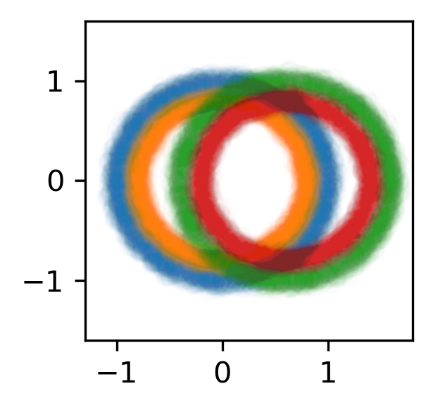
The training dataset with 60,000 data. The 4 classes are shown with different colors, and in addition to the two features shown (on the x/y axes) there are also 4 other usefuless features.

Let’s search for the best model to classify this dataset. Let’s search over these parameters:

• One hyperparameters that control optimal model architecture: hidden_layer_sizes. This can take values that have 12 neurons; for example, 6 neurons in two layers or 4 neurons in 3 layers.

• Six hyperparameters that control finding the optimal model of a particular architecture. This includes hyperparameters such as weight decay and various optimization parameters (including batch size, learning rate and momentum).

Here’s how we’ll configure the two different estimators:

1. “Hyperband” is configured with rule-of-thumb above with n_params = 299 1 and n_examples = 50 * len(X_train).

2. “Incremental” is configured to do the same amount of work as Hyperband with IncrementalSearchCV(..., n_initial_parameters=19, decay_rate=0)

These two estimators are configured do the same amount of computation, the equivalent of fitting about 19 models. With this amount of computation, how do the final accuracies look?

The final validation accuracy over 200 different runs of the estimators above. Out of the 200 runs, the worst HyperbandSearchCV run performed better than 99 of the IncrementalSearchCV runs.

This is great – HyperbandSearchCV looks to be a lot more confident than IncrementalSearchCV. But how fast do these searches find models of (say) 85% accuracy? Experimentally, Hyperband reaches 84% accuracy at about 350 passes through the dataset, and Incremental requires 900 passes through the dataset:

The average accuracy obtained by each search after a certain number of passes through the dataset. The green line is passes through the data required to train 4 models to completion.

“Passes through the dataset” is a good proxy for “time to solution” in this case because only 4 Dask workers are used, and they’re all busy for the vast majority of the search. How does this change with the number of workers?

To see this, let’s analyze how the time-to-completion for Hyperband varies with the number of Dask workers in a separate experiment.

The time-to-completion for a single run of Hyperband as the number of Dask workers vary. The solid white line is the time required to train one model.

It looks like the speedup starts to saturate around 24 Dask workers. This number will increase if the search space becomes larger or if model evaluation takes longer.

1

Approximately 300 parameters were desired; 299 was chosen to make the Dask array chunk evenly

previous

Cross Validation

next

Pipelines and Composite Estimators